Single-Objective with Constraints#
In this tutorial, we will introduce how to optimize a constrained problem with OpenBox.
Problem Setup#
First, define search space and define objective function to minimize. Here we use the constrained Mishra function.
import numpy as np
from openbox import space as sp

def mishra(config: sp.Configuration):
    config_dict = config.get_dictionary()
    X = np.array([config_dict['x%d' % i] for i in range(2)])
    x, y = X[0], X[1]
    t1 = np.sin(y) * np.exp((1 - np.cos(x))**2)
    t2 = np.cos(x) * np.exp((1 - np.sin(y))**2)
    t3 = (x - y)**2

    result = dict()
    result['objectives'] = [t1 + t2 + t3, ]
    result['constraints'] = [np.sum((X + 5)**2) - 25, ]
    return result

params = {
    'float': {
        'x0': (-10, 0, -5),
        'x1': (-6.5, 0, -3.25)
    }
}
space = sp.Space()
space.add_variables([
    sp.Real(name, *para) for name, para in params['float'].items()
])
After evaluation, the objective function returns a dict (Recommended). The result dictionary should contain:
‘objectives’: A list/tuple of objective values (to be minimized). In this example, we have only one objective so the tuple contains a single value.
‘constraints’: A list/tuple of constraint values. Non-positive constraint values (“<=0”) imply feasibility.
Optimization#
After defining the search space and the objective function, we can run the optimization process as follows:
from openbox import Optimizer

opt = Optimizer(
    mishra,
    space,
    num_constraints=1,
    num_objectives=1,
    surrogate_type='gp',
    acq_optimizer_type='random_scipy',
    max_runs=50,
    time_limit_per_trial=10,
    task_id='soc',
)
history = opt.run()
Here we create a Optimizer instance, and pass the objective function and the search space to it. The other parameters are:
num_objectives=1 and num_constraints=1 indicate that our function returns a single value with one constraint.
max_runs=50 means the optimization will take 50 rounds (optimizing the objective function 50 times).
time_limit_per_trial sets the time budget (seconds) of each objective function evaluation. Once the evaluation time exceeds this limit, objective function will return as a failed trial.
task_id is set to identify the optimization process.
Then, opt.run() is called to start the optimization process.
Visualization#
After the optimization, opt.run() returns the optimization history. Or you can call opt.get_history() to get the history. Then, call print(history) to see the result:
history = opt.get_history()
print(history)
+-------------------------+---------------------+
| Parameters              | Optimal Value       |
+-------------------------+---------------------+
| x0                      | -3.172421           |
| x1                      | -1.506397           |
+-------------------------+---------------------+
| Optimal Objective Value | -105.72769850551406 |
+-------------------------+---------------------+
| Num Configs             | 50                  |
+-------------------------+---------------------+
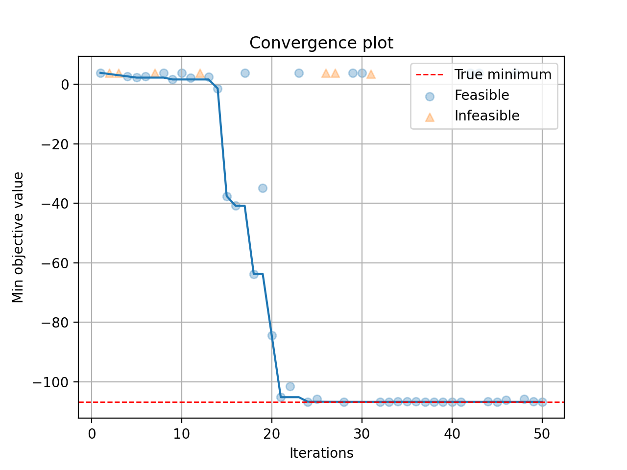
Call history.plot_convergence() to visualize the optimization process:
import matplotlib.pyplot as plt
history.plot_convergence(true_minimum=-106.7645367)
plt.show()